Announcing Updated and Expanded flexAEM Exercise Sets

 Making AnAqSim even easier to learn, and expanding its power

We are happy to announce that, as flexAEM training nears its 10^th year, we have completely updated our series of training exercises. These exercises match the new look and features of AnAqSim Analytic Element Method (AEM) groundwater modeling software, and have been reorganized to make it easier to learn how to build your AnAqSim modeling skills in a stepped and progressive program of training.

In addition, we have added new exercise sets to enhance the speed of building and calibrating an AnAqSim model. These include instructions and example for using the accuracy and spatial data availability of QGIS geospatial analysis software to build your AnAqSim models. And there is a comprehensive introduction that explains and demonstrates how to harness the power of PEST to automatically calibrate and perform parameter uncertainty analyses for your AnAqSim flow models. Both QGIS and PEST are free software that can be obtained from their respective authoring organizations for use with AnAqSim.

Exercises are organized into 15 sets that build in depth and complexity as your training advances (see Figure 1).

 

Figure 1. New reorganized, updated, and expanded flexAEM exercise sets provide a structured way to lead you step by step through the process of learning AEM groundwater flow modeling with AnAqSim.

AEM groundwater modeling holds a number of advantages over numerical techniques like Finite Difference and Finite Element. You don’t have to spend hours or days setting up and tweaking your modeling grid of rectangles or triangles and trying to fit the hydrologic features of your model into that “checkerboard”. You focus on the actual location and geometry of the features themselves, draw them into your model space, and assign them properties. And then when you solve you don’t just get a head value back at your grid block centers or nodes; you can calculate head as a continuous function anywhere in space. This gives you unparalleled accuracy without the computational burden of a super-fine mesh.

The 15 flexAEM exercise sets are ordered from easy to more complex. This allows you to begin with the basics and then progress through more advanced model-building and flow system analysis techniques (see Figure 1). And each set is assembled to contain several exercises that demonstrate the topic, with each exercise containing step-by-step instructions and diagrams, and any needed starting files and basemap files.

This system of self-paced training will have you building a “Hello World” introductory groundwater model in minutes (Figure 2), and can place the efficiency and power of AEM modeling in your hands in days to weeks (Figure 3) depending on how deep you need to go for your initial modeling projects and how much time you can commit.

Figure 2. Simple “Hello World” example lets you build an AnAqSim model in 10 minutes

Figure 3. flexAEM exercises introduce you to AEM modeling concepts and AnAqSim
features such as groundwater flow pathline tracing.

And there is no need to work step-by-step through every exercise, although that can be very helpful in absorbing all that the flexAEM training has to impart. It may speed your progress to start with the basics to understand AEM modeling concepts and the AnAqSim software, and then “skip ahead” to a particular feature or method that you are trying to employ in the model you are developing, read how that is done, and put those tips to use directly into your project model.

Any of the 15 flexAEM exercise sets can be purchased individually, but greater understanding of AnAqSim (and greater savings) can be achieved by purchasing pre-packaged exercise bundles. The entire system consists of over 80 exercises and over 2000 pages of instruction and examples. Purchasing the Ultimate Bundle package gives you all of that at a price that should fit well in any training budget and pays tremendous dividends in the project work that it can support.

In addition, the flexAEM system also makes available software tools to support AnAqSim model building. These include element shape generation software that allows the user to automatically create AnAqSim element vertex locations for a variety of elements line types and shapes, at any scale and any orientation. There is also a set of pre-constructed AnAqSim models that are designed to serve as simple calculator-type tools for designing, or evaluating the performance of, a range of groundwater remediation systems (wells, trenches, slurry walls, caps, etc.).

Please visit the flexAEM website at https://www.flexaem.com/ to view the new updated and enhanced AnAqSim training exercises, and begin adding the ease-of-use, accuracy, flexibility, and power of Analytic Element Method groundwater modeling to your projects today.

AnAqSim River Element with Dry Up Feature

AnAqSim River Element is Different from a MODFLOW River Cell

AnAqSim has a River element that is similar in function to the MODFLOW River Package (or River cell). The AnAqSim River element has a “Dry Up” option that allows the River element to also behave like a MODFLOW Drain cell. We will discuss both modes of River element operation below.

[Note: The AnAqSim Drain/Fracture element is different from a MODFLOW Drain cell; but that is a story for another blog post. For example, the MODFLOW Drain cell has a lower threshold reference head - - an AnAqSim Drain element does not.]

How a River Element Behaves

When creating an AnAqSIm River element, the user specifies a Reference Stage (hydraulic head) in the river, a conductance for the river bed, and also the elevation of the bottom of the river bed (which comes into play in certain head conditions as described below). If the Aquifer Head is above the Reference Stage, groundwater discharges from the aquifer into the river (Figure 1). AnAqSim calculates the groundwater flux per length of river element into the river linesink based on 1) the head difference between the groundwater in the domain at the river location and the river reference stage, and 2) the conductance of the river bed using the following equation:

Q/L = C*(h - stage)                                           (Equation 1)

where conductance, C = (bed Kv * river width) / bed thickness.

Figure 1. Aquifer Head greater than river Reference Stage. Groundwater flows from the aquifer into the river (gaining river).

The greater the calculated Aquifer Head, the greater the groundwater discharge to the river per length of river, as shown by the red-blue dashed line in Figure 2 (see also AnAqSim User Guide):

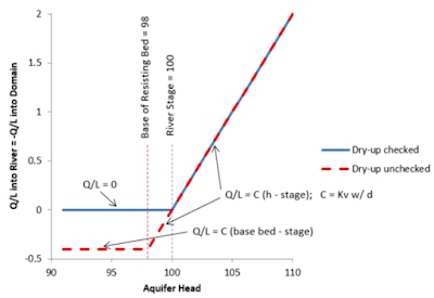Figure 2. River Discharge (Q/L) from the aquifer (positive Q/L) or to the aquifer (negative Q/L) per unit length of River element depending on relationship between calculated aquifer head and specified river reference stage.

 

When the Aquifer Head falls to an elevation equal to the Reference Stage, then flow in or out of the river is zero (as shown in Figure 2 at Aquifer Head equals 100, and in Figure 3).

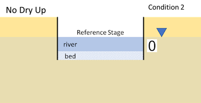Figure 3. Aquifer Head equal to river Reference Stage. No flow occurs between the aquifer and the river.

When the calculated Aquifer Head falls below the river Reference Stage (Aquifer Head = 100 in Figure 2), but is still above the bottom of the river bed material (“Base resisting layer” - - 98 in Figure 2), flow reverses and leakage goes from the river to the aquifer (losing river) (Figure 4). 

As Aquifer Head falls, AnAqSim continues to calculate flow per unit of line length using Equation 1 above, but at a continually decreasing rate (as shown in Figure 2 when Aquifer Head is between 100 and 98, and in Figure 4).

 

Figure 4. Aquifer Head falls below Reference Stage but remains above the bottom of the river bed. River leaks water through the bed to the aquifer (losing river).

This reduction in Aquifer Head values continues until the Aquifer Head falls below the base (bottom) of the river bed material (Figure 5).

At that point, and for any lower aquifer heads, the river element switches from Equation 1 to this equation:

Q/L = C*(base bed - stage)                                (Equation 2)

This means that the Aquifer Head no longer affects the river leakage rate through the bed, since the Aquifer Head is now below the bottom of the bed. Bed leakage is now solely a function of the head drop from the river stage to the elevation of the bottom of the bed, and the bed’s resistance (conductance). With “Dries up” unchecked AnAqSim assumes that there is enough of an upstream water source to keep the water elevation in the river constantly at the Reference Stage. This causes Q/L from Equation 2 to also be constant (flat horizontal line to the left of “Base resisting layer” - - 98 in Figure 2).

Figure 5. Aquifer Head below bottom of river bed (resisting layer). Leakage from river to aquifer is not influenced by Aquifer Head but is controlled by the head drop from the reference stage to the elevation of the river bed through the river bed conductance.

How a River Element Behaves with Dry Up Checked

The AnAqSim river element has a very useful user-selectable “Dry Up” feature. This feature allows a river linesink that is being used to represent a small stream to “dry up” - - i.e. stop accepting water from the aquifer into the river, and do not add water to the aquifer from the river - - when AnAqSim calculates that the Aquifer Head is lower than the river Reference Stage.

The underlying concept here is that the stream is not fed by a large enough upstream source to maintain the user-specified Reference Head. Instead, as groundwater falls below the Reference Head, so too does the stage in the stream. Under those conditions, the stream, which is experiencing zero head gradient between itself and the surrounding aquifer, neither receives nor gives water until the stream completely dries up (when the stage reaches the top of the bed material).

Thus the “Dry Up” condition is more properly understood not as an immediately “dried up” stream (i.e. stream stage at the top of the bed) as soon as the groundwater reaches the same elevation as the Reference Stage, but rather as a “no longer either receives nor gives water” from that reference elevation or lesser, with the stream stage matching the Aquifer Head and no water interchange occurring.

Just as happens for the “no-dry-up” river element, groundwater discharges into the “Dry Up” river element when Aquifer Head is greater than the river Reference Stage (Figure 6).

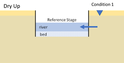Figure 6. Aquifer Head greater than river Reference Stage. Groundwater flows from the aquifer into the river (gaining river).

And similar to the no-dry-up river, when the Aquifer Head falls to an elevation equal to the Reference Stage in the Dry-Up river element (Aquifer Head = 100 in Figure 2), flow in or out of the river is zero (see Figure 2 and Figure 7).

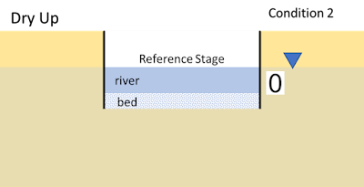Figure 7. Aquifer Head equal to river Reference Stage. No flow occurs between the aquifer and the river.

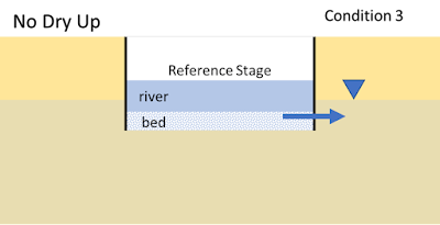
But, differing from the no-dry-up river element, when Aquifer Head falls below the river Reference Stage (but remains above the bottom of the bed), the Dry-Up river element does not give leakage flow to the aquifer (i.e. it is not a losing river) (Figure 8).

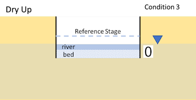Figure 8. Aquifer Head falls below Reference Stage but remains above the bottom of the river bed. Leakage into river remains at zero (because it is assumed that the stream stage cannot be maintained in the small stream and falls to coincide with the head in the aquifer).

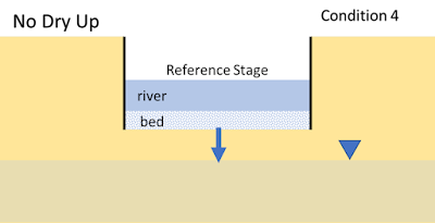
Further, when the Aquifer Head falls below the stream bed bottom elevation, instead of the stream supplying water to the aquifer under Equation 2 above, it yields no water (“dries up”) (Figure 9).

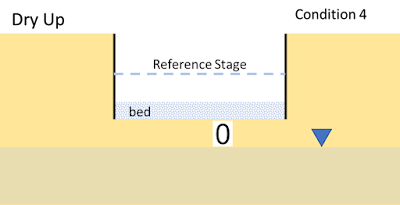Figure 9. Aquifer Head below bottom of river bed (resisting layer). No leakage occurs from the river to the aquifer because under this condition the river is assumed to be completely dried up.

What MODFLOW Does to Represent a River and a Drain

MODFLOW does not have this “Dry Up” capability in the River Package. Instead, MODFLOW handles this condition in two ways:

1.  If the user specifies the river using the River Package, and the groundwater head in a cell falls below the user-specified reference stage, the river continues to flow (does not dry up), and it infiltrates river water to groundwater at a rate determined by the head difference and the bed conductance. This is how the River Package functions, and there is no “Dry Up” option to turn off the infiltration of river water if calculated groundwater head falls below the specified reference stage.

OR

2.  If the user specifies a small river or stream using the Drain Package, and groundwater head in a cell falls below the user-specified reference stage, the stream (drain) dries up and does not infiltrate stream water to groundwater. This is inherently how the Drain functions; there is no checkbox for the user to turn this behavior on or off.

 Conclusion

Thus the AnAqSim River Element, with its “Dry Up” capability, functions as both a traditional MODFLOW River Package feature or a traditional MODFLOW Drain Package feature, depending on how the user sets the “Dries Up” checkbox setting.

So...How Does AnAqSim Compare to MODFLOW?

Here at flexAEM, one of the questions that often comes up is “How does AnAqSim compare to MODFLOW?” Although this question is somewhat broad, and can be interpreted in different ways, two ways in which AnAqSim and MODFLOW can be compared are in their capabilities and their accuracy. As to a comparison of capabilities, AnAqSim includes many of the key features that have made MODFLOW so popular (and one of the most widely used groundwater modeling software programs in the world today). For instance:

• Like MODFLOW, AnAqSim has the ability to incorporate multiple layers into a model, which allows for better representation of more complex aquifer systems. 
• The subdomain method that AnAqSim is based on allows you to apply this mult-layer capability only in the area of interest within a broader, less detailed regional model domain.  This flexible layering scheme is similar to nested grid models that can be generated using more recent versions of MODFLOW, such as MODFLOW-USG and MODFLOW-6.
• The area of the aquifer for which you build an AnAqSim model can be hydraulically linked to extended areas of the aquifer you are analyzing using the same types of specified head, specified flow, or general head boundary conditions that are applied in MODFLOW.
• AnAqSim, like MODFLOW, can simulate both steady-state and transient flow conditions.
• With regard to Transient simulations, similar to MODFLOW, AnAqSim allows the user to specify stress periods and time steps, and vary several different model inputs through time, including aquifer recharge, well pumping rates, and river stages. 
• AnAqSim (like MODFLOW) also allows for the incorporation of anisotropy.
• AnAqSim can be used to trace particle pathlines in three dimensions (which can be done using MODPATH upon generation of a flow field using MODFLOW).
• Like MODFLOW, PEST can be used in conjunction with AnAqSim to automate and greatly streamline the model calibration process (see our Blog post on using PEST with AnAqSim HERE). 

But what about accuracy?  How do modeling results from AnAqSim compare to those generated by MODFLOW?  Since the AEM method is based on exact analytical solutions, whereas MODFLOW uses the finite difference method to approximate those solutions, the answer is that AnAqSim is typically more accurate than MODFLOW. To illustrate this, a simple box model with three pumping wells was generated using AnAqSim and MODFLOW. As shown in Figures 1 and 2 below, the MODFLOW results become increasingly more accurate as the model is further discretized, and to achieve a similar level of accuracy as the results generated by AnAqSim, a grid spacing of 2.5’ x 2.5’ must be utilized in the MODFLOW model, which can be computationally taxing.

Figure 1 – Comparison of simulated head field using AnAqSim and MODFLOW with Variable Grid Spacing

Figure 2 – Comparison of simulated heads using AnAqSim and MODFLOW with Variable Grid Spacing (with MODFLOW grids turned off and heads at pumping wells displayed)

How about particle pathline tracing?  Again, a comparison of particle pathlines generated using AnAqSim and MODFLOW/MODPATH in a model with a “stepped” base elevation indicates that the results match almost exactly (see Figure 3 below).

Figure 3 – Comparison of AnAqSim and MODFLOW particle pathlines with a 5-ft stepped base elevation

For additional comparisons of AnAqSim to MODFLOW (and other analytical solutions), please visit Fitts Geosolutions’ “Checks of AnAqSim” page.As demonstrated above, a comparison of the features and accuracy of results generated by AnAqSim and MODFLOW indicates that AnAqSim incorporates many of the key features and capabilities that make MODFLOW such a versatile, widely used tool, and produces results that are typically more accurate than those generated by MODFLOW. These capabilities make AnAqSim a great alternative to MODFLOW for most simple to moderately complex modeling projects.

AnAqSim Instructional Series Set 8!

With summer in the rear-view mirror and cooler temperatures approaching, there’s never been a better time to hunker down and get back to the basics of AnAqSim with the flexAEM AnAqSim Instructional Series!  In this post we highlight Exercise Set 8, which provides an in-depth look at the key AnAqSim features and tools for constructing groundwater models and analyzing model results. Topics covered in the series include:

• Working with Data Grids
• Solver Settings and Checks
• Model Inspector Tools
• Analysis Tools
• Digitizing Tools
• Editing XML Model Input files
• Exporting Model Data and Graphic results

Although Set 8 explores all these tools and features in detail, there are several in particular that are useful when building models and analyzing results in AnAqSim.

Inspector Tools

The model inspector tools (which are displayed along the left side of the plot view window – see diagram below) allow you to explore flow system conditions at any model location such as saturated thickness, head, specific discharge, layer-to-layer leakage and many more. As you move the cursor over the model, parameters are updated based on the cursor location and current model solution.

Model Inspector Tool displaying parameters of the model

Digitizing Tools

One of the most common ways to begin constructing a model is by importing a basemap and using AnAqSim’s Digitization tools to digitize key features in your model, such as domain boundaries, monitoring wells, lakes and streams, or other internal line boundaries (e.g., an extraction trench associated with a groundwater remediation system). These tools can also be used to accurately position pathline starting locations along lines or within areas. AnAqSim provides instructions on how to digitize any shape, which makes it easy to build any features needed in model construction.

Analysis Tools

AnAqSim’s suite of analysis tools allow the user to develop models with ease, explore model results, and gain important information from the model.  For instance, the Graph Conditions Along a Line feature allows you to create graphs of head, domain elevations, interface elevations, aquifer discharge, or extraction rates along a line chosen by the user. These graphs are useful to view how pathlines will move through the model, check a head profile over a boundary, or check to see if the model is functioning properly. Additional analysis tools allow modelers to create plots of head or drawdown hydrographs, plots of boundary discharges, and plots that display calibration results for the current model solutions.

Graph output from Graph Condition Along a Line tool displaying pathlines, head levels, and domain boundaries.

AnAqSim Instructional Series Exercise Set 8 is a great way to learn how to use these tools and learn helpful tips on model construction (e.g. proper solver settings and editing of XML input files if necessary) to make the best use of AnAqSim’s capabilities.

For further information on the instructional series, or if you would like to purchase the series, please visit flexaem.com.

Using the Drain/Fracture Element – Part 3 of 3: Flow in Bedrock Fracture or Fault Zones

 As described in Part 1 and Part 2 of this series, Drain/Fracture elements are useful internal boundaries for easily modeling a variety of hydrologic features including collector trenches, interconnected ponds, and transmissive fracture or fault zones.

This example will demonstrate the use of a drain/fracture line element to represent a zone of more transmissive fractured or faulted rock within a lower permeability bedrock aquifer.

Discrete Fractures and Fracture Zones

In areas with discrete water-bearing fractures, drain elements can be incorporated into an AnAqSim model to direct flow along the higher conductance fracture(s). This capability can be useful when looking at groundwater contours and drawdown; however, particle pathlines cannot be tracked through drain/fracture elements, making interpretation of groundwater flow paths difficult, especially when multiple drain/fracture elements are combined.

To address this pathline issue, the use of separate fractured domains with anisotropy (different K1_horizontal and K2_horizontal values and an Angle_K1_to_x_axis aligned with the fracture strike) is recommended when using particle pathline tracing to evaluate model results is important. As shown in the examples below, the drawdown caused by pumping within a fractured region represented by discrete fractures is nearly identical to the drawdown caused by pumping within a fractured region represented by an anisotropic domain with representative bulk hydraulic conductivities along strike and perpendicular to strike (Fig 1 and Fig 2).

Fig 1. Drawdown caused by extraction well located within a fractured region represented by discrete fractures

Fig 2. Drawdown caused by extraction well located within the equivalent anisotropic porous media fractured region

While the two fractured zone representations both provide similar drawdown plots, they do not produce equivalent particle pathlines to the pumping well located within the fractured region. Pathlines within the equivalent anisotropic porous media agree with the flow of groundwater, predominantly along strike within fractures (Fig 4), while the pathlines tracked from the well located within the discrete fractures appear to flow across strike rather than along it (Fig 3). This is because pathlines that intercept the drain/fracture elements are terminated, so only pathlines that aren’t captured by the drains are tracked perpendicular to the hydraulic gradient.

Fig 3. Pathlines tracked to an extraction well located within a fractured region represented by discrete fractures

Fig 4. Pathlines tracked to an extraction well located within the equivalent anisotropic porous media fractured region

Pathlines in the discrete fracture model primarily terminate at the closest fractures on either side of the well, while the pathlines in the equivalent anisotropic porous media model travel along strike while within the fractured region. The equivalent anisotropic porous media model produces a more representative capture zone and thus may be more useful when determining capture zones for wells within fractured regions.

Summary

Drain/fracture elements can easily produce hydraulic head contours resulting from discrete fractures, pipes, or karst zones located within an aquifer and can effectively represent drawdown resulting from pumping near those drain/fracture elements. If capture zones are desired, drain/fracture elements are not the right choice because the particles are not tracked along the line elements. Instead, representative anisotropic domains may be more appropriate for representing capture zones. The discrete drain/fracture elements can still play a role in developing the representative anisotropic domain if the number, aperture (width), and hydraulic conductivity of the fractures is approximately known. This will allow a model with an anisotropic domain to be fit to the discrete fracture model (by adjusting K1_horizontal, K2_horizontal, and Angle_K1_to_x_axis in the fracture domain window).

Tips and Tricks

• Use more closely spaced nodes near the end of drain/fracture line elements where the boundary condition is changing rapidly if head contours are not smooth.
• Using equations within excel can be useful to quickly set up multiple line boundaries that are aligned parallel to each other.

The models used in the above examples are available in this zipped file. The above examples require the full version of AnAqSim to solve. AnAqSim is available from Fitts Geosolutions.

Using the Drain/Fracture Element – Part 2 of 3: Connecting a Series of Ponds

 As described in Part 1 of this series, Drain/Fracture elements are useful internal boundaries for easily modeling a variety of hydrologic features including collector trenches, interconnected ponds, and transmissive fracture or fault zones.

This example will demonstrate the use of a drain/fracture line element to connect a series of ponds in such a way that water flows freely between the ponds and keeps them hydraulically linked regardless of additions or withdrawals from one of the ponds.

A pond in direct communication with the aquifer

In this example, a series of three ponds are in direct communication with the aquifer, and each pond is connected by a small stream. Because the ponds are in direct communication with the aquifer, groundwater is able to easily flow through the ponds as if they were a high hydraulic conductivity unit within the aquifer. And because the three ponds are linked by streams, the water level within all three ponds is nearly identical. This simple model uses five drain elements with high conductance values to represent the three ponds and two connecting streams (Fig 1). The Drain elements conduct water along their length effectively causing the three ponds to have roughly equal surface elevations (Fig 2).

Fig 1. Three ponds (represented by circular drain elements) connected by short stream segments (represented by linear drain elements).

Fig 2. Groundwater elevations in the vicinity of the ponds and connecting stream. Note that the easy flow among the ponds transmitted by the stream drain segments maintains the elevation of water in the ponds, and elevation of the adjacent groundwater in the aquifer, very close to 90 ft msl.

Increasing or decreasing the conductance of the drain elements can be used to control the elevations of the ponds relative to each other. A higher conductance will cause the three pond surface elevations to be closer together, while using a lower conductance will cause the three pond surface elevations to be further apart. If we increase the conductance of the model shown in the previous figure by a factor of 10, we can see that the 90-foot contour extends around the first pond, rather than cutting between the first and second ponds (Fig 3).

Fig 3. Increasing drain element conductance in the model enhances the hydraulic connection among the ponds, and all elevations more closely approximate 90 ft msl.

Similarly, decreasing the conductance of the original model by a factor of 100 causes additional contours above and below the 90-foot contour to separate the ponds, resulting in a larger hydraulic gradient between the three ponds.

Fig 4. Decreasing drain element conductance in the model reduces the hydraulic connection between the ponds and the aquifer, and from pond to pond, causing a significant decreasing head condition through the pond system from left to right.

In the above examples, the conductances of all five drains used to represent the ponds and connecting streams were changed uniformly, but each drain segment can be adjusted individually to better represent observed conditions.

Summary

Drain/fracture elements can easily represent ponds and networks of ponds that are in direct communication with the aquifer and hydraulically linked to each other. Using a high conductance for the drain/fracture elements (on the order 1 Million to 10 Million ft²/d) will cause ponds to have approximately equal surface elevations. Ponds at different surface elevations can be manual matched by adjusting the conductance of some or all of the drain/fracture elements to match observed surface water elevations. Representing ponds and streams using drain/fracture elements assumes that the surface water bodies are in direct communication with the aquifer and are neither extracting nor supplying water to the aquifer system. If the ponds are in-fact a source or sink in the aquifer system, spatially variable area source/sinks should be used for separate pond domains and river line boundaries should be used for the streams.

Tips and Tricks

• For larger ponds, adding one or more drain lines within the interior of the pond will help to maintain heads across the entire pond.

• To represent water extraction from within one of the ponds, a well or constant flux line element can be placed within the pond at a specified extraction rate.

The models used to in the above examples are available in this zipped file. Both model files are solvable using either AnAqSimEDU (the free version) or the full version of AnAqSim. Both versions are available from the Fitts Geosolutions.

Using Drain/Fracture Line Boundaries in AnAqSim – Part 1 of 3: Collector Trench Example

Drain/Fracture elements in AnAqSim are useful internal line boundaries that conduct water at a high rate compared to the surrounding domain.  They can be used to easily model a variety of linear hydrologic features including:

• Trench drains that collect water in a high permeability trench and direct flow towards an extraction well

• Ponds in direct communication with the aquifer where modeling pond responses to model stresses is desired

• Discrete fractures or fractured zones

This example will demonstrate the use of drain/fracture line elements to represent a collector trench for groundwater dewatering or remediation, and parts 2 and 3 will focus on modeling ponds and fractures using drain/fracture line elements.

AnAqSim employs these drain/fracture elements as line boundaries with specified conductance (hydraulic conductivity * width) that can transmit large volumes of water. Note that drain/fracture elements in AnAqSim are different than drain boundaries employed in MODFLOW. Drain/fracture elements do not remove water from the model and the user does not supply a reference elevation. If you are trying to simulate a MODFLOW type drain boundary in AnAqSim, it is best to use the River element with the “Dries_up” box ticked. Note also that, while the drain/fracture feature is referred to as a boundary in AnAqSim, it is created using a line dipole function and should not be used to form an external domain boundary, nor should it contact or be joined to an external domain boundary - it is strictly an internal boundary.

Drain/fracture elements can be employed in any instance where hydraulic features can be conceptualized as a thin linear zone with a greater hydraulic conductivity than the surrounding aquifer. While that zone may have a physical width in the real aquifer, as for example in the case of a trench, the mathematical line boundary has zero width. This prevents any pathline tracing along these features as they transmit flow along their orientation. This limitation, along with other tips for implementation, will be discussed in the following example.

Trench Drains

Trench drains with extraction sumps or wells are useful remedial technologies to consider when evaluating remedial options at sites with impacted groundwater, or for certain dewatering applications. AnAqSim allows for rapid simulation of trench drains and extraction wells using either trench drain domains separated from the aquifer by interdomain boundaries or drain/fracture elements with an equivalent conductance (Kx * w) within the aquifer.

Previously, we have represented trench drains as separate domains in flexAEM exercises and calculators (available from the flexAEM website); this is an effective strategy that allows for particle tracing within the drain, but it can be time consuming to input the nodes along the edge of the drain (especially for complex drain geometries that do not align with the x and y axes). Drain/Fracture elements have are easier to input because only a single line is required (although care should be taken near the ends of trench drains to add additional nodes where the boundary condition changes rapidly). Additionally, a node is required at locations that correspond to wells pumping within the trench drain, otherwise the pumping will not be properly conveyed to the trench drain.

The examples below show a trench drain represented with a separate domain (Fig 1) and a trench drain represented using the drain/fracture element (Fig 2). Both examples have three pumping wells located within the trench drain pumping at 4,000 ft³/d or approximately 30,000 gpd. The trench drain is 4 feet wide with a hydraulic conductivity of 1,000 ft/d; this corresponds to a conductance of 4,000 ft²/d for the drain/fracture element.

Fig 1. Trench Drain Represented by a High Hydraulic Conductivity Domain

Fig 2. Trench Drain Represented by a Drain/Fracture Element

Notice that the two trench drain representations yield identical head contours (compare Figs 3 and 4), but the separate trench drain domain model produces a much more complete representation of the particle pathlines (Fig 3)  that represent the capture zones of the three wells. Although the drain/fracture element model does not allow particles to travel along the length of the drain (Fig 4), the particles that are shown represent the overall extent of the trench drain and extraction well capture zone.

Fig 3. Trench Drain Represented by a Separate High Hydraulic Conductivity Domain

Fig 4. Trench Drain Represented by a Drain/Fracture Element

Summary

Drain/fracture elements are useful features in AnAqSim that can be utilized to rapidly model trench drains used for capturing impacted water or dewatering. Modeling the dewatering effect of a trench drain and sump, without the need for particle pathline tracing is an efficient use of drain/fracture elements since it allows the user to save time when digitizing the trench drain.

Tips and Tricks

• In the above example, near the ends of the trench drain and near the three wells, the spacing of drain/fracture element nodes was decreased to less than 1-foot to provide greater resolution where the boundary condition changes rapidly. If you are experiencing jagged contours near the drain, try decreasing the node spacing to see if this helps to smooth the contours.

• If you have used drain/fracture elements in your model and you would like to perform particle pathline tracing, try adding a line of pathlines that trace backwards from immediately upstream of the drain/fracture element and another line of pathlines that trace forward immediately downstream of the drain/fracture element. This will give you a fairly good understanding of the flow directions on either side of the drain/fracture element, but will not indicate how far particles travel along the drain/fracture element before reentering the aquifer.

The models used to in the above examples are available in this zipped file. Both model files are solvable using either AnAqSimEDU (the free version) or the full version of AnAqSim. Both versions are available from the Fitts Geosolutions.